Show the code
pacman::p_load( sf, sfdep, tmap, tidyverse, knitr)This in-class introduces an alternative R package to spdep package. The package is called sfdep. According to Josiah Parry, the developer of the package, “sfdep builds on the great shoulders of spdep package for spatial dependence. sfdep creates an sf and tidyverse friendly interface to the package as well as introduces new functionality that is not present in spdep. sfdep utilizes list columns extensively to make this interface possible.”
Five R packages will be used for this in-class exercise, they are: sf, sfdep, tmap, tidyverse, and knitr.
Using the steps you learned in previous lesson, install and load sf, tmap, sfdep, tidyverse and knitr packages into R environment.
pacman::p_load( sf, sfdep, tmap, tidyverse, knitr)For the purpose of this in-class exercise, the Hunan data sets will be used. There are two data sets in this use case, they are:
Hunan, a geospatial data set in ESRI shapefile format, and
Hunan_2012, an attribute data set in csv format.
Using the steps you learned in previous lesson, import Hunan shapefile into R environment as an sf data frame.
hunan <- st_read(dsn = "data/geospatial", layer = "Hunan")Reading layer `Hunan' from data source
`W:\widyayutika\ISSS624\In-class_Exercise\In-class_Ex2\data\geospatial'
using driver `ESRI Shapefile'
Simple feature collection with 88 features and 7 fields
Geometry type: POLYGON
Dimension: XY
Bounding box: xmin: 108.7831 ymin: 24.6342 xmax: 114.2544 ymax: 30.12812
Geodetic CRS: WGS 84Using the steps you learned in previous lesson, import Hunan_2012.csv into R environment as an tibble data frame.
hunan2012 <- read_csv("data/aspatial/Hunan_2012.csv")Using the steps you learned in previous lesson, combine the Hunan sf data frame and Hunan_2012 data frame. Ensure that the output is an sf data frame.
hunan_GDPPC <- left_join(hunan,hunan2012)%>%
select(1:4, 7, 15)In order to retain the geospatial properties, the left data frame must the sf data.frame (i.e. hunan)
Using the steps you learned in previous lesson, plot a choropleth map showing the distribution of GDPPC of Hunan Province.
The choropleth should look similar to ther figure below.
tmap_mode("plot")
tm_shape(hunan_GDPPC) +
  tm_fill("GDPPC",
          style = "quantile",
          palette = "Blues",
          title = "GDPPC") +
  tm_borders(alpha = 0.5) +
  tm_layout(main.title = "Distribution of GDP per capita by district, Hunan Province",
            main.title.position = "center",
            main.title.size = 1.2,
            legend.height = 0.45,
            legend.width = 0.35,
            frame = TRUE) +
  tm_compass(type="8star", size = 2) +
  tm_scale_bar() +
  tm_grid(alpha =0.2)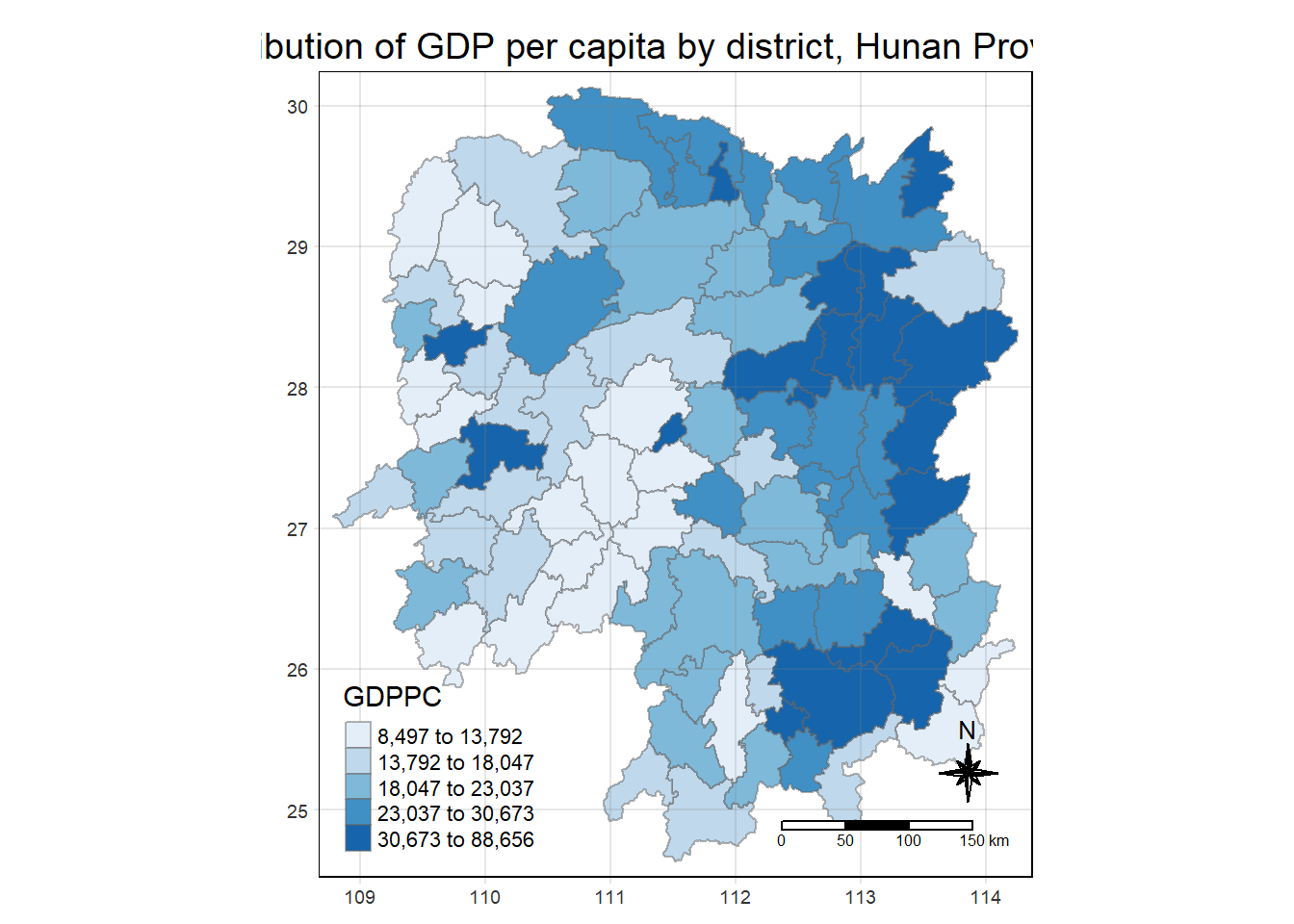
By and large, there are two types of spatial weights, they are contiguity wights and distance-based weights. In this section, you will learn how to derive contiguity spatial weights by using sfdep.
Two steps are required to derive a contiguity spatial weights, they are:
identifying contiguity neighbour list by st_contiguity() of sfdep package, and
deriving the contiguity spatial weights by using st_weights() of sfdep package
In this section, we will learn how to derive the contiguity neighbour list and contiguity spatial weights separately. Then, we will learn how to combine both steps into a single process.
In the code chunk below st_contiguity() is used to derive a contiguity neighbour list by using Queen’s method.
wm_q <- hunan_GDPPC %>%
  mutate(nb = st_contiguity(geometry),
         wt = st_weights(nb, style = "W"),
.before=1).before=1 -> put nb and wt at the front of the tibble dataset
By default, queen argument is TRUE. If you do not specify queen = FALSE, this function will return a list of first order neighbours by using the Queen criteria. Rooks method will be used to identify the first order neighbour if queen = FALSE is used.
The code chunk below is used to print the summary of the first lag neighbour list (i.e. nb) .
summary(wm_q$nb)Neighbour list object:
Number of regions: 88
Number of nonzero links: 448
Percentage nonzero weights: 5.785124
Average number of links: 5.090909
Link number distribution:
1 2 3 4 5 6 7 8 9 11
2 2 12 16 24 14 11 4 2 1
2 least connected regions:
30 65 with 1 link
1 most connected region:
85 with 11 linksThe summary report above shows that there are 88 area units in Hunan province. The most connected area unit has 11 neighbours. There are two are units with only one neighbour.
To view the content of the data table, you can either display the output data frame on RStudio data viewer or by printing out the first ten records by using the code chunk below.
wm_qSimple feature collection with 88 features and 8 fields
Geometry type: POLYGON
Dimension: XY
Bounding box: xmin: 108.7831 ymin: 24.6342 xmax: 114.2544 ymax: 30.12812
Geodetic CRS: WGS 84
First 10 features:
nb
1 2, 3, 4, 57, 85
2 1, 57, 58, 78, 85
3 1, 4, 5, 85
4 1, 3, 5, 6
5 3, 4, 6, 85
6 4, 5, 69, 75, 85
7 67, 71, 74, 84
8 9, 46, 47, 56, 78, 80, 86
9 8, 66, 68, 78, 84, 86
10 16, 17, 19, 20, 22, 70, 72, 73
wt
1 0.2, 0.2, 0.2, 0.2, 0.2
2 0.2, 0.2, 0.2, 0.2, 0.2
3 0.25, 0.25, 0.25, 0.25
4 0.25, 0.25, 0.25, 0.25
5 0.25, 0.25, 0.25, 0.25
6 0.2, 0.2, 0.2, 0.2, 0.2
7 0.25, 0.25, 0.25, 0.25
8 0.1428571, 0.1428571, 0.1428571, 0.1428571, 0.1428571, 0.1428571, 0.1428571
9 0.1666667, 0.1666667, 0.1666667, 0.1666667, 0.1666667, 0.1666667
10 0.125, 0.125, 0.125, 0.125, 0.125, 0.125, 0.125, 0.125
NAME_2 ID_3 NAME_3 ENGTYPE_3 County GDPPC
1 Changde 21098 Anxiang County Anxiang 23667
2 Changde 21100 Hanshou County Hanshou 20981
3 Changde 21101 Jinshi County City Jinshi 34592
4 Changde 21102 Li County Li 24473
5 Changde 21103 Linli County Linli 25554
6 Changde 21104 Shimen County Shimen 27137
7 Changsha 21109 Liuyang County City Liuyang 63118
8 Changsha 21110 Ningxiang County Ningxiang 62202
9 Changsha 21111 Wangcheng County Wangcheng 70666
10 Chenzhou 21112 Anren County Anren 12761
geometry
1 POLYGON ((112.0625 29.75523...
2 POLYGON ((112.2288 29.11684...
3 POLYGON ((111.8927 29.6013,...
4 POLYGON ((111.3731 29.94649...
5 POLYGON ((111.6324 29.76288...
6 POLYGON ((110.8825 30.11675...
7 POLYGON ((113.9905 28.5682,...
8 POLYGON ((112.7181 28.38299...
9 POLYGON ((112.7914 28.52688...
10 POLYGON ((113.1757 26.82734...The print shows that polygon 1 has five neighbours. They are polygons number 2, 3, 4, 57,and 85.
One of the advantage of sfdep over spdep is that the output is an sf tibble data frame.
Using the steps you learned in previous lesson, display nb_queen sf tibble data frame in a table display.
kable(head(wm_q,n=10))| nb | wt | NAME_2 | ID_3 | NAME_3 | ENGTYPE_3 | County | GDPPC | geometry |
|---|---|---|---|---|---|---|---|---|
| 2, 3, 4, 57, 85 | 0.2, 0.2, 0.2, 0.2, 0.2 | Changde | 21098 | Anxiang | County | Anxiang | 23667 | POLYGON ((112.0625 29.75523… |
| 1, 57, 58, 78, 85 | 0.2, 0.2, 0.2, 0.2, 0.2 | Changde | 21100 | Hanshou | County | Hanshou | 20981 | POLYGON ((112.2288 29.11684… |
| 1, 4, 5, 85 | 0.25, 0.25, 0.25, 0.25 | Changde | 21101 | Jinshi | County City | Jinshi | 34592 | POLYGON ((111.8927 29.6013,… |
| 1, 3, 5, 6 | 0.25, 0.25, 0.25, 0.25 | Changde | 21102 | Li | County | Li | 24473 | POLYGON ((111.3731 29.94649… |
| 3, 4, 6, 85 | 0.25, 0.25, 0.25, 0.25 | Changde | 21103 | Linli | County | Linli | 25554 | POLYGON ((111.6324 29.76288… |
| 4, 5, 69, 75, 85 | 0.2, 0.2, 0.2, 0.2, 0.2 | Changde | 21104 | Shimen | County | Shimen | 27137 | POLYGON ((110.8825 30.11675… |
| 67, 71, 74, 84 | 0.25, 0.25, 0.25, 0.25 | Changsha | 21109 | Liuyang | County City | Liuyang | 63118 | POLYGON ((113.9905 28.5682,… |
| 9, 46, 47, 56, 78, 80, 86 | 0.1428571, 0.1428571, 0.1428571, 0.1428571, 0.1428571, 0.1428571, 0.1428571 | Changsha | 21110 | Ningxiang | County | Ningxiang | 62202 | POLYGON ((112.7181 28.38299… |
| 8, 66, 68, 78, 84, 86 | 0.1666667, 0.1666667, 0.1666667, 0.1666667, 0.1666667, 0.1666667 | Changsha | 21111 | Wangcheng | County | Wangcheng | 70666 | POLYGON ((112.7914 28.52688… |
| 16, 17, 19, 20, 22, 70, 72, 73 | 0.125, 0.125, 0.125, 0.125, 0.125, 0.125, 0.125, 0.125 | Chenzhou | 21112 | Anren | County | Anren | 12761 | POLYGON ((113.1757 26.82734… |
Using the steps you just learned, derive a contiguity neighbour list using Rooks’ method.
wm_r <- hunan_GDPPC %>%
  mutate(nb = st_contiguity(geometry, queen=FALSE),
         wt = st_weights(nb, style = "W"),
.before=1)There are times that we need to identify high order contiguity neighbours. To accomplish the task, st_nb_lag_cumul() should be used as shown in the code chunk below.
Using the steps you just learned, derive a contiguity neighbour list using lag 2 Queen’s method.
nb2_queen <-  hunan_GDPPC %>%
  mutate(nb = st_contiguity(geometry),
         nb2 = st_nb_lag_cumul(nb, 2),
         .before = 1)
Note that if the order is 2, the result contains both 1st and 2nd order neighbors as shown on the print below.
nb2_queenSimple feature collection with 88 features and 8 fields
Geometry type: POLYGON
Dimension: XY
Bounding box: xmin: 108.7831 ymin: 24.6342 xmax: 114.2544 ymax: 30.12812
Geodetic CRS: WGS 84
First 10 features:
nb
1 2, 3, 4, 57, 85
2 1, 57, 58, 78, 85
3 1, 4, 5, 85
4 1, 3, 5, 6
5 3, 4, 6, 85
6 4, 5, 69, 75, 85
7 67, 71, 74, 84
8 9, 46, 47, 56, 78, 80, 86
9 8, 66, 68, 78, 84, 86
10 16, 17, 19, 20, 22, 70, 72, 73
nb2
1 2, 3, 4, 5, 6, 32, 56, 57, 58, 64, 69, 75, 76, 78, 85
2 1, 3, 4, 5, 6, 8, 9, 32, 56, 57, 58, 64, 68, 69, 75, 76, 78, 85
3 1, 2, 4, 5, 6, 32, 56, 57, 69, 75, 78, 85
4 1, 2, 3, 5, 6, 57, 69, 75, 85
5 1, 2, 3, 4, 6, 32, 56, 57, 69, 75, 78, 85
6 1, 2, 3, 4, 5, 32, 53, 55, 56, 57, 69, 75, 78, 85
7 9, 19, 66, 67, 71, 73, 74, 76, 84, 86
8 2, 9, 19, 21, 31, 32, 34, 35, 36, 41, 45, 46, 47, 56, 58, 66, 68, 74, 78, 80, 84, 85, 86
9 2, 7, 8, 19, 21, 35, 46, 47, 56, 58, 66, 67, 68, 74, 76, 78, 80, 84, 85, 86
10 11, 14, 15, 16, 17, 18, 19, 20, 21, 22, 23, 70, 71, 72, 73, 74, 82, 83, 86
NAME_2 ID_3 NAME_3 ENGTYPE_3 County GDPPC
1 Changde 21098 Anxiang County Anxiang 23667
2 Changde 21100 Hanshou County Hanshou 20981
3 Changde 21101 Jinshi County City Jinshi 34592
4 Changde 21102 Li County Li 24473
5 Changde 21103 Linli County Linli 25554
6 Changde 21104 Shimen County Shimen 27137
7 Changsha 21109 Liuyang County City Liuyang 63118
8 Changsha 21110 Ningxiang County Ningxiang 62202
9 Changsha 21111 Wangcheng County Wangcheng 70666
10 Chenzhou 21112 Anren County Anren 12761
geometry
1 POLYGON ((112.0625 29.75523...
2 POLYGON ((112.2288 29.11684...
3 POLYGON ((111.8927 29.6013,...
4 POLYGON ((111.3731 29.94649...
5 POLYGON ((111.6324 29.76288...
6 POLYGON ((110.8825 30.11675...
7 POLYGON ((113.9905 28.5682,...
8 POLYGON ((112.7181 28.38299...
9 POLYGON ((112.7914 28.52688...
10 POLYGON ((113.1757 26.82734...In this section, you will learn how to compute Local Moran’s I of GDPPC at county level by using local_moran() of sfdep package.
lisa <- wm_q %>%
  mutate(local_moran = local_moran(
    GDPPC, nb, wt, nsim = 99),
    .before = 1) %>%
  unnest(local_moran)
The output of local_moran() is a sf data.frame containing the columns ii, eii, var_ii, z_ii, p_ii, p_ii_sim, and p_folded_sim.
ii: local moran statistic
eii: expectation of local moran statistic; for localmoran_permthe permutation sample means
var_ii: variance of local moran statistic; for localmoran_permthe permutation sample standard deviations
z_ii: standard deviate of local moran statistic; for localmoran_perm based on permutation sample means and standard deviations
p_ii: p-value of local moran statistic using pnorm(); for localmoran_perm using standard deviatse based on permutation sample means and standard deviations
p_ii_sim: For localmoran_perm(), rank() and punif() of observed statistic rank for [0, 1] p-values using alternative=
p_folded_sim: the simulation folded [0, 0.5] range ranked p-value based on crand.py of pysal
skewness: For localmoran_perm, the output of e1071::skewness() for the permutation samples underlying the standard deviates
kurtosis: For localmoran_perm, the output of e1071::kurtosis() for the permutation samples underlying the standard deviates.
unnest() of tidyr package is used to expand a list-column containing data frames into rows and columns.
In this code chunk below, tmap functions are used prepare a choropleth map by using value in the ii field.
tmap_mode("plot")
tm_shape(lisa) +
  tm_fill("ii") +
  tm_borders(alpha = 0.5) +
  tm_view(set.zoom.limits = c(6,8)) +
  tm_layout(main.title = "local Moran's I of GDPPC",
            main.title.size = 0.8)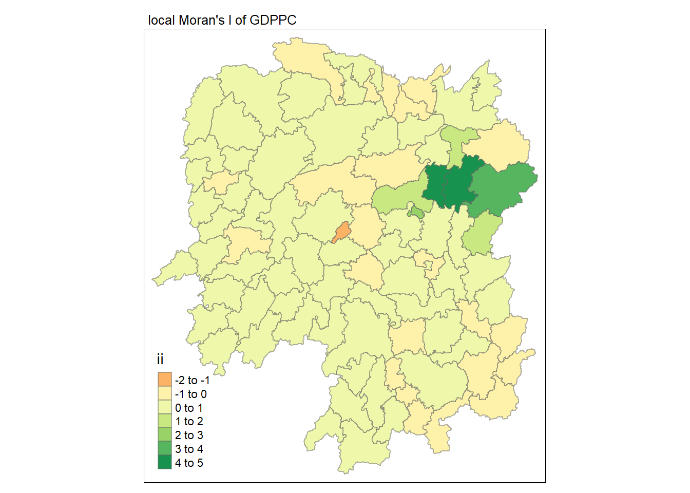
In the code chunk below, tmap functions are used prepare a choropleth map by using value in the p_ii_sim field.
tmap_mode("plot")
tm_shape(lisa) +
  tm_fill("p_ii_sim") +
  tm_borders(alpha = 0.5) +
   tm_layout(main.title = "p-value of local Moran's I",
            main.title.size = 0.8)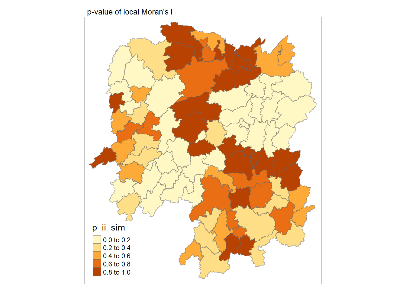
For p-values, the appropriate classification should be 0.001, 0.01, 0.05 and not significant instead of using default classification scheme.
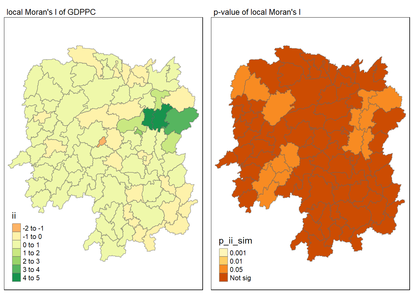
For effective comparison, it will be better for us to plot both maps next to each other as shown below.
tmap_mode("plot")
map1 <- tm_shape(lisa) +
  tm_fill("ii") +
  tm_borders(alpha = 0.5) +
  tm_view(set.zoom.limits = c(6,8)) +
  tm_layout(main.title = "local Moran's I of GDPPC",
            main.title.size = 0.8)

map2 <- tm_shape(lisa) +
  tm_fill("p_ii_sim",
          breaks = c(0, 0.001, 0.01, 0.05, 1),
              labels = c("0.001", "0.01", "0.05", "Not sig")) +
  tm_borders(alpha = 0.5) +
  tm_layout(main.title = "p-value of local Moran's I",
            main.title.size = 0.8)

tmap_arrange(map1, map2, ncol = 2)